
Binomial Distributions
Reviewing your toolbox
Welcome to the first of our quarterly newsletters for 2023!
You may recall, the blog posts in 2022 followed the Six Sigma DMAIC (Define, Measure, Analyze, Improve, Control) methodology therefore for 2023, we wanted to dive a bit deeper into some select tools from both the Six Sigma and Lean toolboxes. If there are any specific tools you would like highlighted in a post this year please email lstuart@ezsigmagroup.com and we will be sure to include it.
Without further ado, we shale begin our discussion with Binomial Distributions.
In normal distributions, we could calculate probabilities using the table of “areas under the curve”. The normal distribution, however, is a representation of continuous type data. The binomial distribution results from trials where there are only two possible outcomes.
Since these types of trials characterize discrete (attribute) data, such as “defect versus no defect”, we can apply binomial probability. If the binomial distribution approximates the (bell-shape) normal distribution, we can then calculate probabilities using the table of areas under the normal curve.
What does that mean?
As suggested by the prefix “bi” which signifies “two”, the binomial distribution describes the possible number of times a particular event or outcome will occur in a sequence of observations or trials.
This type of event is binary, in that it may or may not occur. Common examples of this would be the tossing of a coin to see how many times it lands “heads-up” or rolling a die to see how often the “number 4” appears. These are success\failure, yes\no, pass\fail responses. In our work, either a defect is present, or it is not.
Now, this may seem quite simple to you right now... I flip a coin once and I can know that either heads will turn up, or it won’t... it has a 50% chance... or does it?
What if you flipped the coin ten times? Would you always see 5 heads out of each set of 10 tries? Conduct you own test right now by repeating this experiment 4 times, each trial consisting of 10 tosses of the coin. Each occurrence of “heads” can be represented by the value 1.
What if you were to repeat a trial, but this time flip the coin 100 times. How would the results change? How does probability figure in something as simple as the toss of a coin, and what should we understand about this concept when conducting our six sigma projects, (or when you are attending a casino).
What is important is to understand how probability is reflected in the binomial distribution therefore, our focus is not on memorizing the math, but understanding the concept and application.
The “Heart” of the Calculation
When a coin is tossed, a card drawn from a deck, (or a student guesses on a multiple-choice test), they all have something in common.
In each case, the events;
- can only have one of two possible results (we could say “dichotomous”, but that would be pretentious!).
- are independent (a preceding event does not influence the subsequent event(s).
- are randomly selected (there is no bias in the outcome or selection)
- are mutually exclusive (the occurrence of one event excludes the possibility of the other event – can’t be both)
With this in mind, we can now have a quick look at the binomial probability of observing r outcomes in n number of trials:
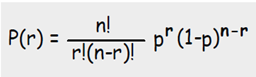
Where p(r) is the probability of exactly r successes or outcomes, n is the number of events, and p is the probability of success for any one trial.
Don’t be intimidated by this expression. You do not have to memorize it, only understand how it works.
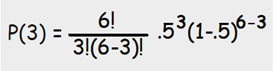
Let’s take our example of the coin toss. What would be the probability of observing exactly 3 heads if a fair coin is flipped 6 times?
- A fair coin (or test) has no bias – that is, either result has equal chance of being selected. There is no influence on the outcome.
Let’s do an example with the following number from a coin toss…
n = 6 (number of events)
r = 3 (the exact number of successful outcomes we want to see)
p = .5 (the coin is fair, so heads has a 50% chance of being observed)
Now, let’s complete the formula…
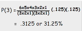
We’ve seen this formula before except for the exclamation marks – what do they mean?
The exclamation mark indicates factorial notation. 6! means 6 x 5 x 4 x 3 x 2 x 1. Your calculator should have a factorial notation button that will make this easier. 6! = 720.
So, let’s simplify this one more time...
The Binomial Distribution
The results can be illustrated in graphical form, presenting a distribution curve whose shape may not be that unfamiliar to you.
The first distribution represents that same trial we have just calculated the probability on: p = .5, n = 6, r = 3
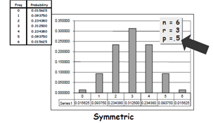
Notice that the probability indicated for observing three heads out of six tosses of the coin is .3125. In addition, you may be thinking that this looks a lot like the normal distribution. We’ll address that further on in this post.
What if we were to change the probability estimate from .5 to something else. The results of this change are shown below.
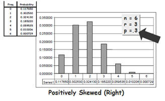
Notice how the distribution is skewed positively to the right, and that the probability of observing 3 heads has been reduced from .3125 to .18522. The highest probability for the occurrence of “heads” is now 2 out of six, since the probability for 2 is .32413.
The distribution no longer resembles the normal curve.
In real life, we may need to make probability estimates using large numbers. While not always possible, it is advantageous to use the normal distribution to approximate a binomial distribution.
Applications of the Binomial Distribution
In this post we have mentioned coin tosses and students guessing at multiple-choice tests, but the binomial distribution has practical applications. It is commonly used in quality control (estimating defects), public opinion surveys, medical research, and estimating insurance casualty claims.
Another situation you may relate to is the reservation process for the airline industry. If, on average, 7% of reservations are “no-shows”, you may want to take more reservations than there are available seats. That way, after netting out the “no-shows”, you will still have a full flight. If you are willing to take a 5% risk of not having enough seats for those who show up, how many reservations can you take in excess of the 200 seats to stay within that allowable risk?
Sampling Without Replacement
Before concluding this post, we will touch briefly on the issue of sampling with or without replacement. As suggested at the start of this post, the binomial distribution requires that you sample with replacement.
To sample without replacement is handled by what is referred to as the hypergeometric distribution. However, as long as the population size is much larger (20 x or more) than the sample size, we can use the binomial distribution. In this instance, we would be approximating the hypergeometric distribution with the binomial distribution.
Summary
We have discussed that the binomial distribution describes the possible number of times that a given event will occur over a series of observations. It uses discrete (attribute) data where there can only be two possible outcomes, yes\no, pass\fail, good\bad, etc.
Our review identified the fact that for a binomial distribution to be applied, the events must also be independent, randomly selected, and mutually exclusive.
We understand that the shape of the binomial distribution is described by two parameters, the number of values for N and the probability assigned to a specific outcome being observed (p).
We can now use this knowledge to estimate the probability of a specific number of events occurring, but to determine the cumulative probability of a range of events, we can use the normal distribution to approximate the binomial distribution, and using the resultant Z value and assign a probability estimate based on the area under the normal curve.
For further information on Binomial Distribution or other Lean Six Sigma tools feel free to reach out to info@ezsigmagroup.com
" I believe that the Binomial Theorem and a Bach Fugue are, in the long run, more important than all the battles in history" - James Hilton (English novelist 1900-1954)
"Life is good for only two things, discovering mathematics and teaching mathematics" - Simeon-Denis Poisson (French scientist 1781-1840)